Build From Scratch
Create the graph and wire the four shader checkpoints, camera, and SetEnvironment.
Follow these steps in a blank TiXL project using the supplied HLSL checkpoints. Use TiXL 4.4.0.4 alpha to match the node names and screenshots.
Download the project and four shader checkpoints. Keep the extracted reference nearby for comparison. To open the finished graph directly, use Quick Start.
Get oriented
The workspace. The Graph View holds the operators and their connections. Select one operator to edit its inputs in Parameters. The Output View shows the selected operator’s result when it can be previewed. Right-click empty space in Graph View to search for and add an operator. The Symbol Library lets you browse what is available. Assets is where you find the project’s textures and HLSL files.
Operators and wires. An operator is a node that does one job. A texture operator produces an image, a value operator produces a number, and a draw operator produces a command for the renderer to run. Drag from an output socket to the receiving input. In this tutorial, Cloud Panorama → Image A means the Image A input on the operator named Cloud Panorama. When an input accepts multiple connections, follow the order in the table or screenshot.
How to check your work. Build one numbered step at a time and compare the Output View with its checkpoint. If selecting a node still shows the old result, check the pin in the Output View toolbar. Click it to follow your selection again. Save the project once the checkpoint works.
1. Start with a blank graph
The starting graph has no operators or connections.
- Choose TiXL → New Project… and give the project a different name from the reference project. Right-click an empty spot in Graph View. Type CustomPixelShader into the node search that opens, then select the stock result from Lib.image.use. Select the new node and enter Cloud Panorama in the instance name field at the top of Parameters.

After choosing the result, the stock Custom Pixel Shader appears where you opened the search. The graph label changes when you name the instance.
- In your project folder, create Assets/weather/volume. Copy the four HLSL files from the archive’s Checkpoints folder into it. Copy CloudNoiseAtlas.dds from the finished project’s Assets/weather/volume folder into the same destination. In TiXL’s Assets panel, expand your project and then weather → volume to check that the files are indexed. The screenshots show the capture project name. Use the package name for the project you created.
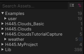
Find your own project package in Assets and expand its weather folder.
- Set Resolution to 2048 × 1024 and Texture Format to R16G16B16A16_Float. The 2:1 image holds a full sphere, and the float format retains sun values above 1 for bloom and lighting.

At the bottom of Parameters, enter both resolution values and choose the float format from the dropdown.
- Scroll down in Parameters to Template File. If the field is hidden, expand Additional Options… or switch the Parameters panel to show all inputs. Click the current value and type 01-Directions.hlsl. Select the matching result under your project’s weather/volume path. The … button beside the value opens the Assets browser if you need to locate the file. Clear the example text from Shader Code. Leave Additional Code empty. Each checkpoint supplies a complete pixel shader through Template File.

Check that the search result belongs to your project and that the selected value ends in weather/volume/01-Directions.hlsl. Use the same field to load each later checkpoint.
- Select Cloud Panorama to see its output. If the output pane is pinned to a different node, click its pin icon to unpin it. To match the graph below, expose the shader’s Texture Output as a graph output named Panorama. The shader can also be previewed directly while building.
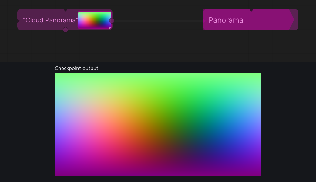
Checkpoint 1 has a single CustomPixelShader. The preview on the right is the direction debug view.
Checkpoint. You should see a false-color panorama. The left and right edges meet at the same longitude, the middle row is the horizon, and the top is straight up.
Build the panorama
At each checkpoint, select Cloud Panorama to see its flat 2:1 image. The camera and environment wiring come after the four shader checkpoints.
2. Add the atmosphere and the HDR sun
- Add LinearGradient and wire its texture into Cloud Panorama → Image A. Set Width to 1 and Rotate to 0, as in the reference. Set Resolution to 8 × 512 and Texture Format to R16G16B16A16_Float. Add the seven gradient stops listed below, using alpha 1 for each. In the shader this is t0, sampled at the ray’s polar angle.
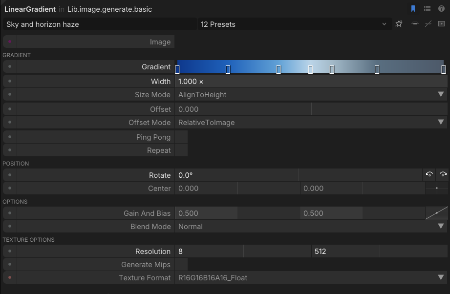
The handles on the Gradient row mark the seven stops in the table. Set the texture resolution near the bottom.
- Add FloatsToBuffer and connect Buffer → Cloud Panorama → Constant Buffers. It is the first custom buffer and appears as b2. Add twelve Value operators from Types.Values. Enter one number in each operator’s Float field and connect its Result to Params, in the order below. You can replace groups of constants with Vector2Components and Vector4Components later to make the controls easier to edit.
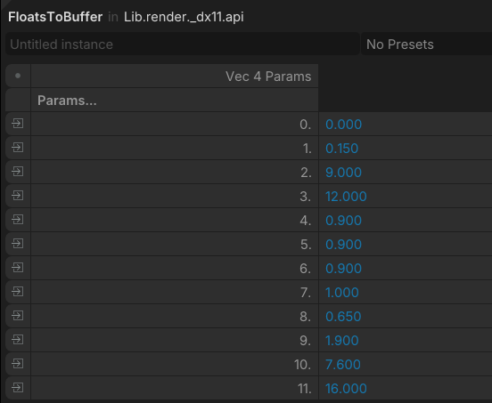
TiXL numbers these rows from 0. Row 0 corresponds to position 1 in the table. The blue values come from connected operators.
- Switch Template File to 02-SkyAndSun.hlsl. Start with Time Of Day = 16.

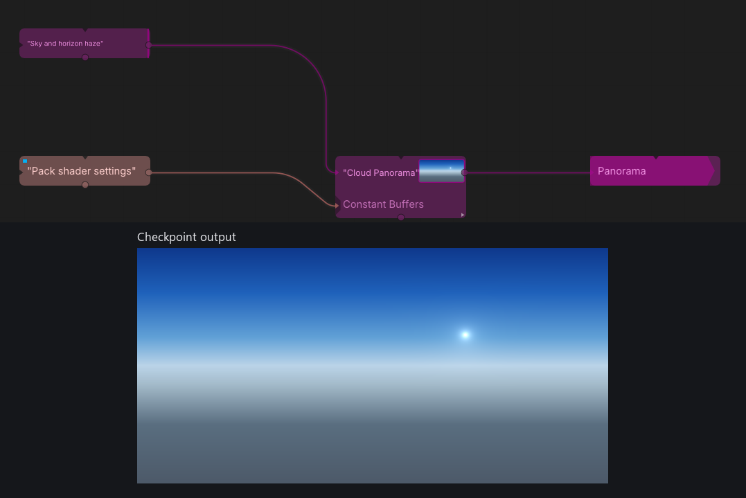
Checkpoint 2 adds a daylight texture and a settings buffer. The shader still draws only the atmosphere and sun.
| Gradient position | RGB |
|---|---|
| 0.00 | (0.055, 0.22, 0.55) |
| 0.19 | (0.12, 0.38, 0.73) |
| 0.38 | (0.38, 0.63, 0.84) |
| 0.50 | (0.73, 0.83, 0.91) |
| 0.58 | (0.64, 0.73, 0.79) |
| 0.75 | (0.35, 0.43, 0.50) |
| 1.00 | (0.30, 0.35, 0.41) |
| Positions in Params | Values to connect in order |
|---|---|
| 1–4 | Sun yaw 0, sun path height 0.15, cloud scale 9, sun radiance 12 |
| 5–8 | Cloud tint RGBA 0.9, 0.9, 0.9, 1 |
| 9–12 | Stratus base 0.65, cumulus base 1.9, cirrus base 7.6, time of day 16 |
Keep the full 12-float buffer even during the sky-only checkpoint. The order matches CloudView in the shader. Reordering two cables changes what the shader reads even when both cables carry floats. The two sun coordinates, scale and radiance fill one four-float register. Tint fills the second. The three altitudes and hour fill the third.
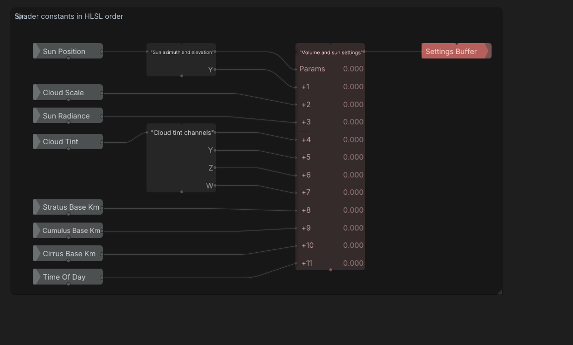
Inside Pack shader settings. Vector2Components splits the sun controls and Vector4Components splits cloud tint. Read the connections from top to bottom. The isolated group preview shows unevaluated values, so enter the numbers from the table above.
Checkpoint. Scrub Time Of Day toward 17.85. The sun drops toward the horizon and the sky turns warm. Return to 16 and set Sun Radiance to 0. The disc and halo disappear while the atmospheric gradient remains. Restore radiance to 12 for the cloud pass.
3. Build the cloud inputs and render cumulus
- Add LoadImage and load CloudNoiseAtlas.dds. Connect its texture to Cloud Panorama → Image B (t1). The atlas holds 64 noise slices in an 8 × 8 grid for stratus and cumulus.
AtlasSlicesamples XY inside one tile, andVolumeNoiseinterpolates between slices along Z. Leave the atlas in its original DDS format and dimensions so the lookup stays aligned.

Use the Path field’s asset search to select the DDS from your own project.
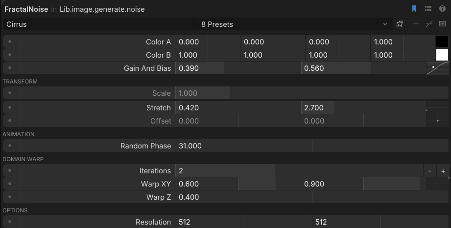
- Add three FractalNoise operators named Cumulus, Stratus, and Cirrus. Use black for Color A and white for Color B, with alpha 1 on both. Set Resolution to 512 × 512 and Iterations to 2 on all three. Then enter the layer settings below.
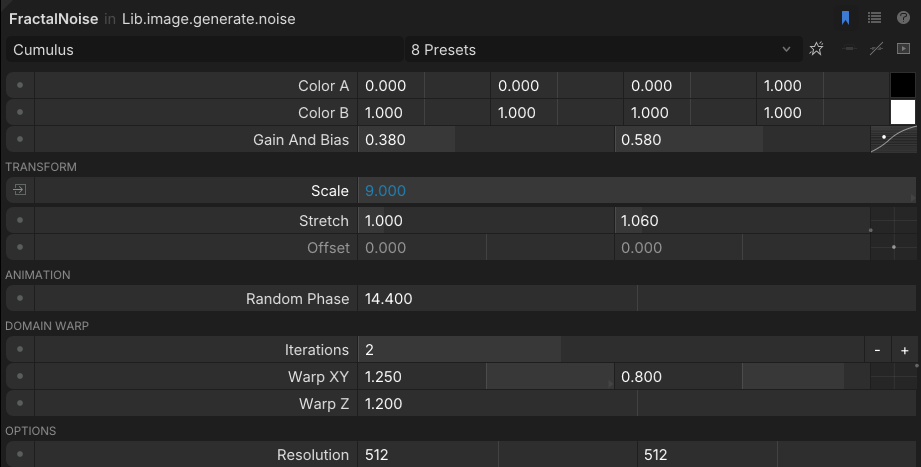
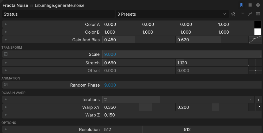
Connected blue values in the reference come from Cloud Scale. Enter the table values on your loose graph.
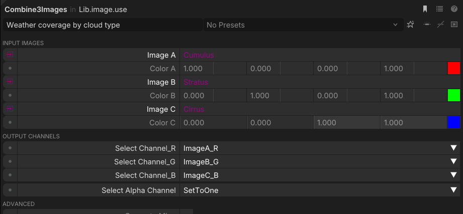
- Feed cumulus into Combine3Images → Image A, stratus into Image B, and cirrus into Image C. Set Select Channel R to Image A R, G to Image B G, and B to Image C B. These are the selectors used by the reference. Wire the output to SrvFromTexture2d → Texture. Connect Shader Resource View → Cloud Panorama → Shader Resources as the first extra texture. It becomes t3.

- Set the shader’s A to 0.62 and B to 0.82. Leave C and D at 0 for this step. Switch to 03-Cumulus.hlsl.


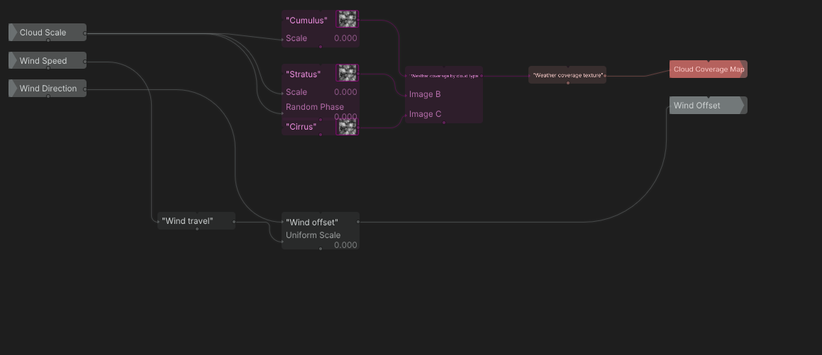
Inside Cloud Maps and Wind. The upper branch packs coverage masks into RGB. The lower branch supplies the wind offset used in step 4.
| Layer | Scale | Random Phase | Stretch | Warp XY | Warp Z | Gain and Bias |
|---|---|---|---|---|---|---|
| Cumulus | 9 | 14.4 | (1, 1.06) | (1.25, 0.8) | 1.2 | (0.38, 0.58) |
| Stratus | 9 | 9 | (0.66, 1.12) | (0.35, 0.2) | 0.15 | (0.45, 0.62) |
| Cirrus | operator default | 31 | (0.42, 2.7) | (0.6, 0.9) | 0.4 | (0.39, 0.56) |
The reference wires the shared Cloud Scale into Scale for cumulus and stratus, and into Random Phase for stratus. Use the constants in the table first, then expose the shared control when you group the graph.
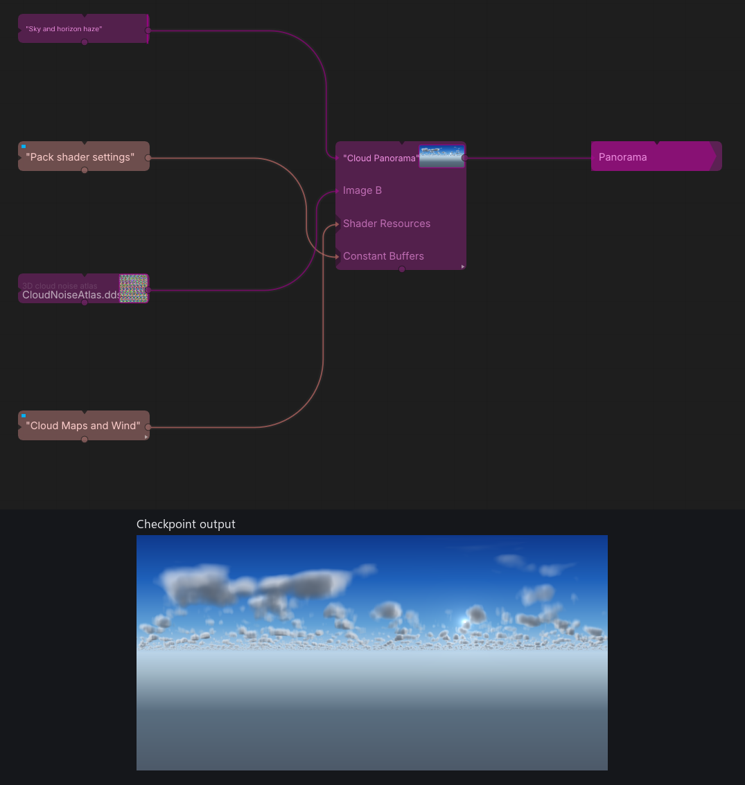
Checkpoint 3 adds the density inputs and shows one volumetric layer. Shader Resources carries the coverage SRV.
| CustomPixelShader input | Value read by the shader |
|---|---|
| Offset | Wind offset, start at (0, 0) |
| A | Cloud cover 0.62 |
| B | Cumulus blend 0.82 |
| C | Stratus blend 0 for this checkpoint |
| D | Cirrus blend 0 for this checkpoint |
Checkpoint. Cumulus should appear above the horizon. Set A to 0 for a clear sky, then bring it back up. Turn Sun Radiance down with the clouds still visible. The direct illumination should fade and the ambient cloud fill should remain.
4. Add stratus, cirrus, and wind
- Switch to 04-CloudVolume.hlsl. Leave A = 0.62 and B = 0.82, then set C = 0.34 and D = 0.50. The shader integrates low stratus, mid-level cumulus, and high cirrus in that order. All three share the same accumulated light and transmittance.


- Change one blend at a time and leave the other two at zero to check its shape and height. Restore the mix, then try changing the three altitude values in the buffer.
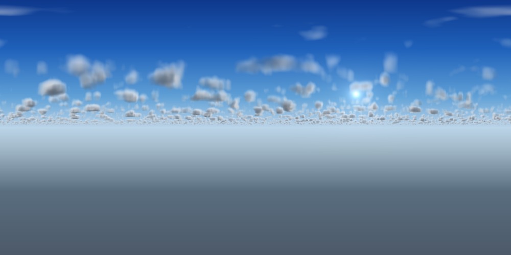
Cumulus only with B = 0.82 and C = D = 0.
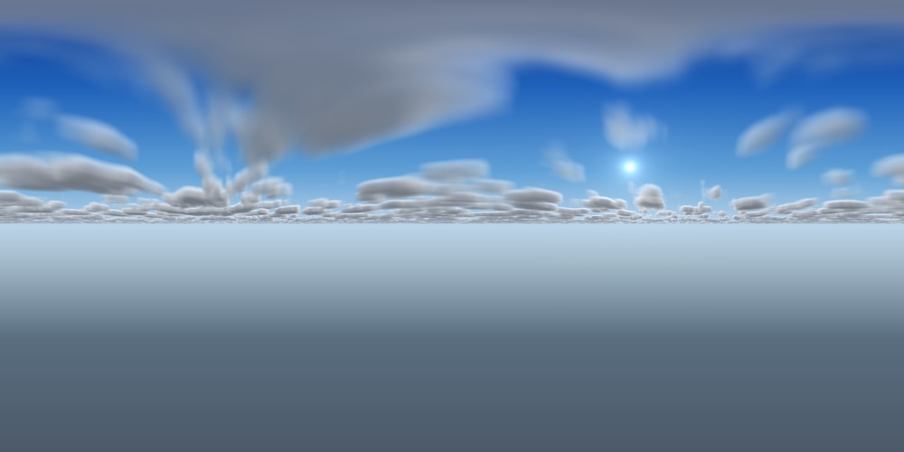
Stratus only with C = 1 and B = D = 0.
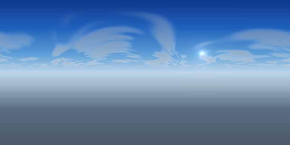
Cirrus only with D = 1 and B = C = 0. The thin streaks curve as they drift with the wind and fade as they recede toward the horizon.
- For moving clouds, add Time, set Mode to Runtime, Units to Secs, and Speed Factor to 0.025. Connect its output to ScaleVector2 → Uniform Scale. Set the direction vector A to (0.36, 0.24) and leave B at (1, 1). Connect the result to the shader’s Offset.


After entering these vectors, connect Time to Uniform Scale.
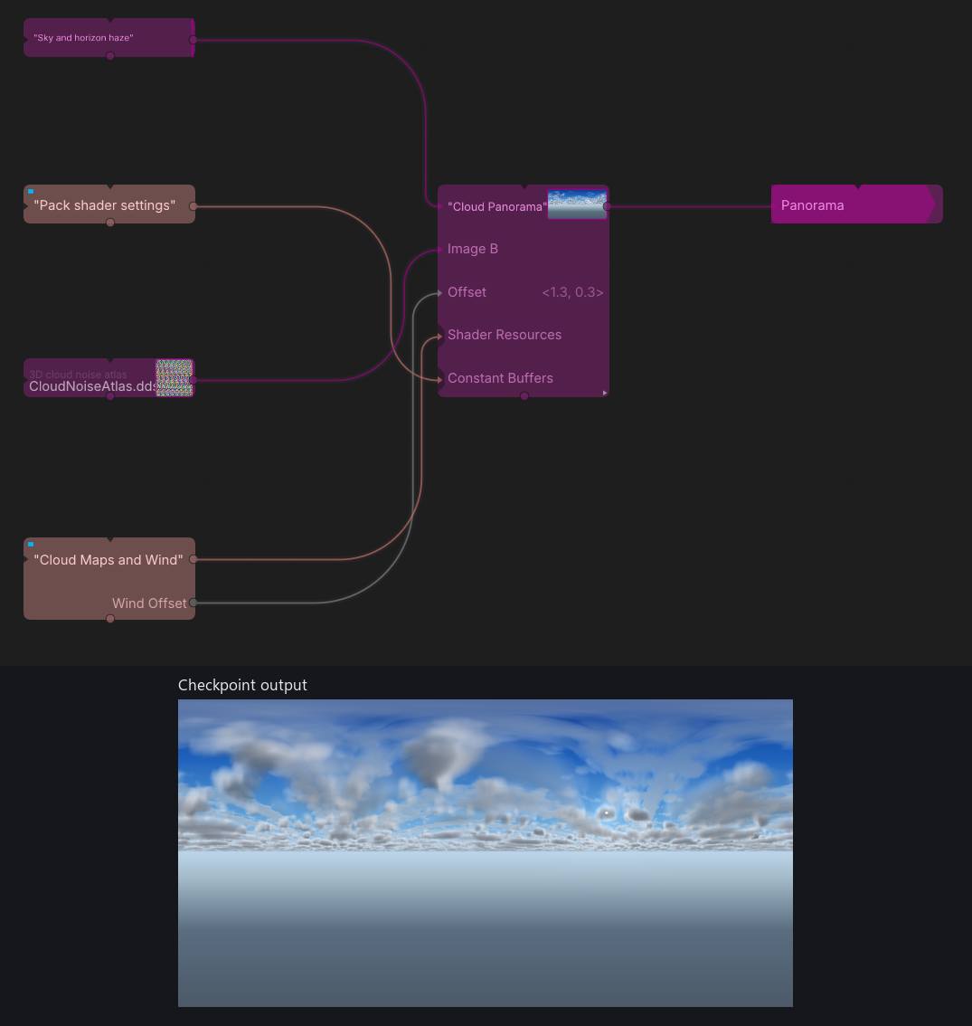
Checkpoint 4 uses the same shader inputs as checkpoint 3 and adds the wind connection. A through D control cover, cumulus, stratus, and cirrus.
The shader applies a different speed multiplier to each layer. The high cirrus should move faster than low stratus.
Checkpoint. Low stratus should spread into a sheet, cumulus should have thicker bodies, and cirrus should sit higher. Freeze wind by setting the Time speed factor to zero while comparing lighting changes.
Render the sky and light a scene
The shader makes a 2D panorama. The next steps convert it into a cubemap, which stores the sky on six faces so the renderer can look up a color by direction. The camera sees one view of that sky through the dome. SetEnvironment uses a second cubemap to light meshes.
5. Turn the panorama into a visible sky
- Connect Cloud Panorama → Texture Output to TextureToCubeMap → Image. Set its face resolution to 1024.

- Add SphereMesh with a radius of −500. Connect it to DrawMeshUnlit → Mesh, and connect the cubemap to DrawMeshUnlit → Texture. Enable Use Cube Map. Disable Enable Z Test and Enable Z Write on this background draw.

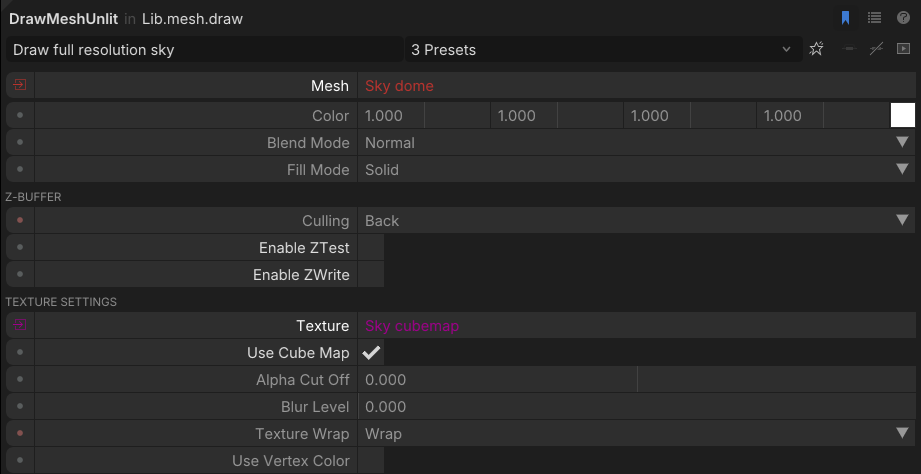
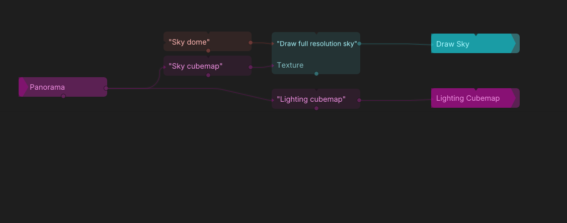
The 1024-pixel-per-face cubemap feeds DrawMeshUnlit. The lower cubemap is prepared for the lighting branch in step 6.
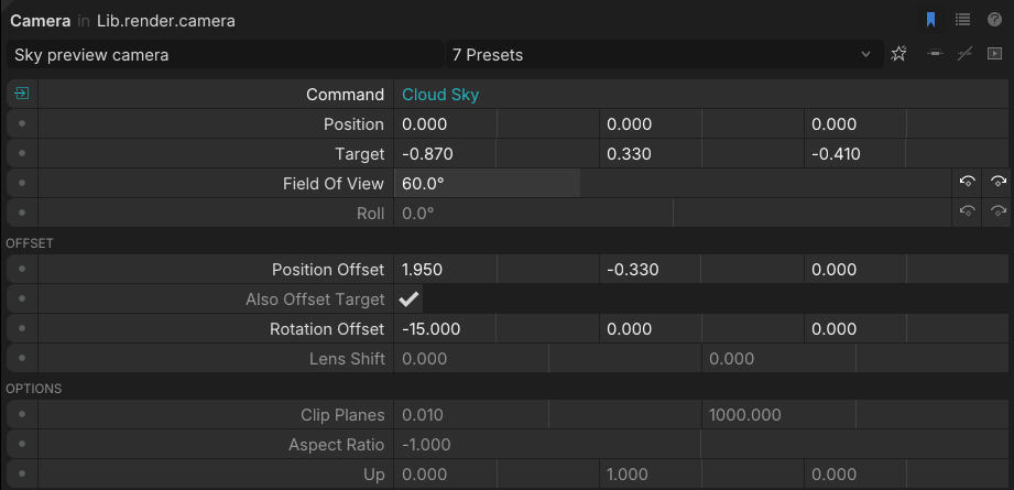
- Connect DrawMeshUnlit → Output to Camera → Command, then Camera → Output to RenderTarget → Command. Put the camera at (0, 0, 0), set its target to (−0.87, 0.33, −0.41), and set Field Of View to 60°. Use R16G16B16A16_Float on the render target and enable Clear and With Depth Buffer. To match the reference framing, set Position Offset to (1.95, −0.33, 0), enable Also Offset Target, and set Rotation Offset to (−15, 0, 0).
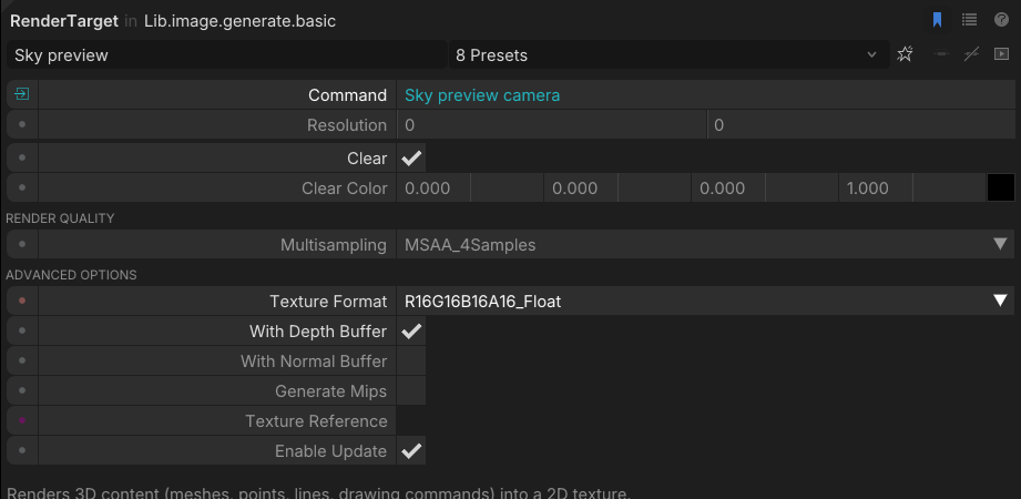
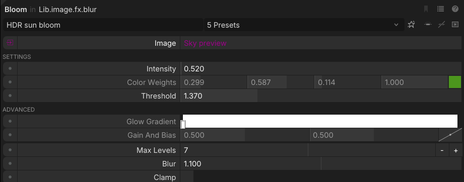
- For the display, connect RenderTarget → Color Buffer through Bloom and then ToneMapping. Start with bloom threshold 1.37 and intensity 0.52, and tone-mapping exposure 0.92 in ACES mode. Select and pin the tone-mapped preview while editing the shader.
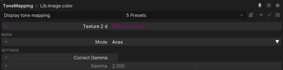
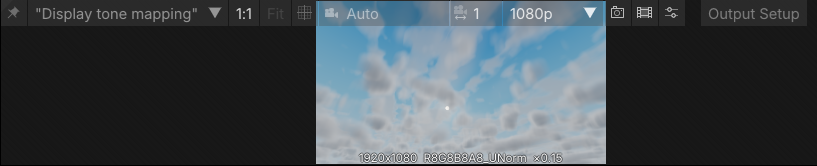
With Display tone mapping selected, click the pin icon immediately left of its name.

The completed preview chain. The Cloud Sky group supplies the draw command assembled in step 6.
Checkpoint. Turn the camera toward the horizon and then tilt it up. The clouds should wrap continuously. At hour 16 the starting camera angle should put the sun in view. Bloom and tone mapping belong on the preview path after the camera render.
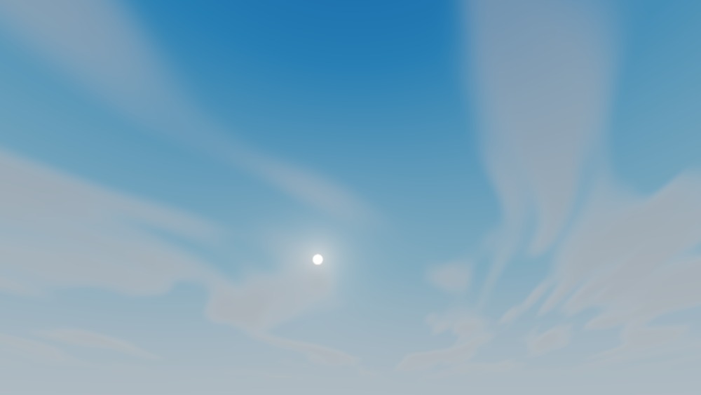
The same isolated cirrus layer viewed through the camera. The panorama above shows all directions flattened into one image.
6. Wire SetEnvironment for scene lighting
Add a second TextureToCubeMap fed by the same HDR panorama. Set its face resolution to 256. Use it for lighting while the 1024-face cubemap continues to draw the dome.

| From | To |
|---|---|
| Cloud Panorama texture | Lighting TextureToCubeMap → Image |
| Lighting cubemap | SetEnvironment → Texture |
| Optional lit scene command | SetEnvironment → Sub Tree |
| DrawMeshUnlit → Output | Execute → Command, first |
| SetEnvironment → Output | Execute → Command, second |
| Execute → Output | Camera → Command, replacing the direct dome cable |
Set SetEnvironment → Render Background to off because the dome draws the background. Enable Update Live so changes to the panorama update the illumination. Start with Exposure = 0.92. In the reference graph the lighting capture also uses Quality Factor = 0.12.
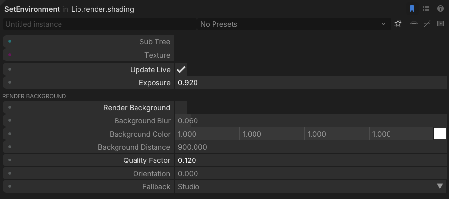
Enter these values on SetEnvironment before promoting them to controls.
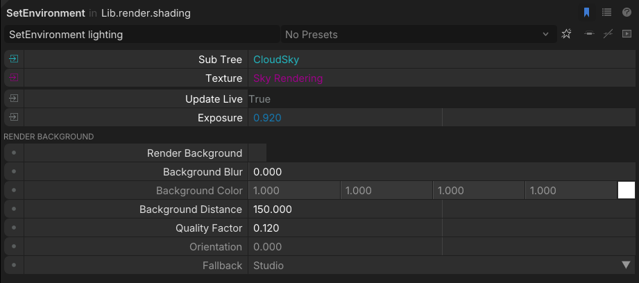
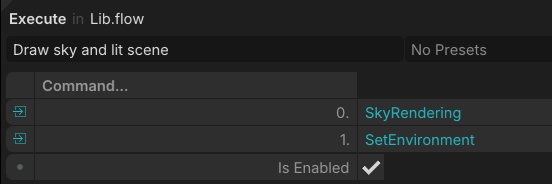
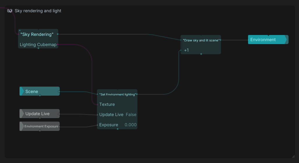
The two command cables into Execute establish draw order. The dome is drawn first, and SetEnvironment lights its optional scene subtree. The connected settings take their live values from the parent graph.
Checkpoint. The sky-only preview should look the same after adding this branch. To see the lighting itself, add a small SphereMesh and a stock DrawMesh with a rough material. Connect the sphere to DrawMesh → Mesh, place it in front of the camera, and connect the draw command to SetEnvironment → Sub Tree. Change Time Of Day or the environment’s Exposure. The mesh lighting should respond independently of the dome. Feed SetEnvironment from the HDR cubemap before bloom and tone mapping so the illumination retains the panorama’s radiance.
7. Organize the finished graph
- Keep the loose graph working before grouping. Add separate value nodes for the parameters you want to expose. Give the nodes descriptive names such as Cloud Cover, Cumulus Blend, Sun Radiance, and Time Of Day. Wire each value node to its destination before you group anything.
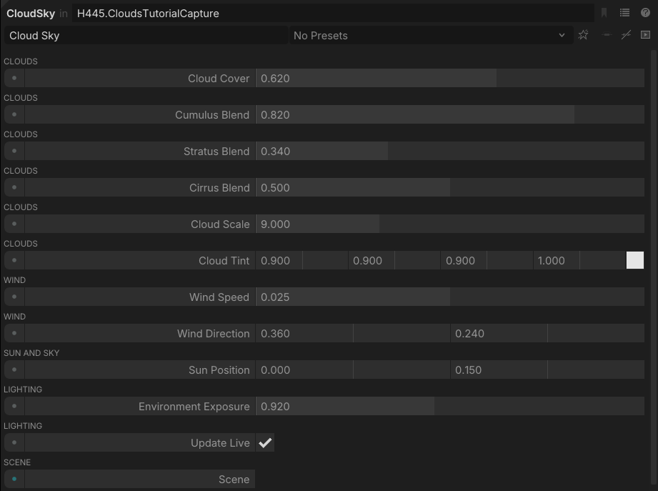
These are the exposed controls you are building. Wire your own value sources to the loose operators first.
- Select the coverage and wind operators. Right-click a selected operator and open Symbol Definition → Combine into New Type…. Enter Cloud Maps and Wind as the group’s name. Keep the control sources outside the selection. Cables crossing the selection become group inputs or outputs. Confirm the two outputs carry the coverage SRV and the wind vector.
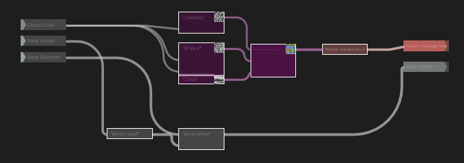
White outlines mark the operators to include. The left-hand control sources and right-hand outputs stay outside the selection.
- Group the constants and vector-splitter operators into Pack shader settings, leaving the editable control sources outside. Keep the 12 input cables in the same order at FloatsToBuffer. Then group the HDR pixel shader and its input textures into Cloud Panorama.
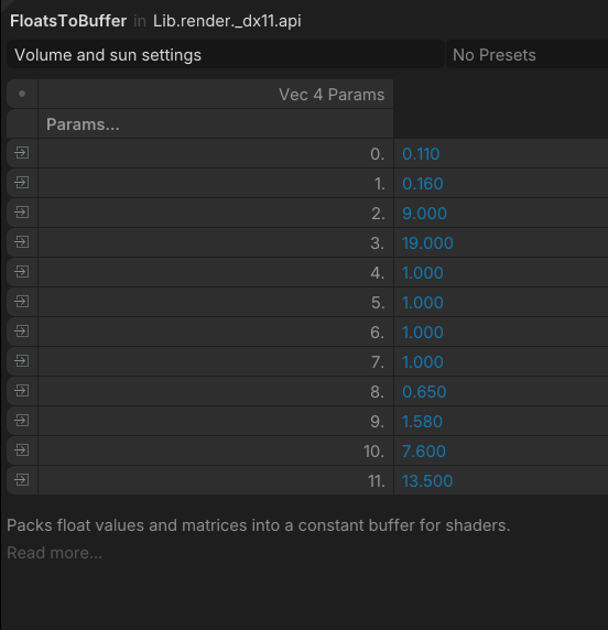
The isolated reference group shows its own defaults. Compare the connection order to step 2, then verify the numbers from the parent graph.
- Group the cubemap converters, sphere mesh, and unlit dome draw into Sky Rendering. Its two outputs should be a dome draw command and a lighting cubemap texture. Keep SetEnvironment and Execute visible in the Cloud Sky group so you can follow how the draw commands are scoped.
- Compare your graph with the download. With the preview pinned, change Cloud Cover, Time Of Day, and Sun Radiance individually. The coverage, sun direction, and direct lighting should respond independently.
Troubleshoot the graph
| Symptom | Check |
|---|---|
| The preview is blank | Select the shader for the flat preview or the tone-mapping output for the camera preview. Check Template File and shader errors. |
| The panorama is visible but the clouds are missing | Verify the DDS on Image B, the coverage SRV as the first extra shader resource, and that A and at least one layer blend are above zero. |
| Sun position, brightness, or altitudes respond to the wrong control | Compare all 12 FloatsToBuffer connections with the table. The buffer assigns values by connection position. |
| The dome looks correct but the mesh lighting stays flat | Make sure the mesh uses a lit material, runs inside SetEnvironment → Sub Tree, and receives the live HDR lighting cubemap. |
The screenshots are from TiXL. Some show isolated parameter entry, and others show the same settings once their inputs are connected in the reference graph.
The finished graph groups the matching stages under Cloud Maps and Wind, Cloud Panorama, Sky Rendering, and Cloud Sky.